Micromagnetic simulations

Micromagnetic simulations are computational methods used to model the behavior of magnetic materials at the microscale. They are also widely used in the study and design of magnetic devices, such as magnetic recording media, magnetic memory devices, and spintronic devices. These simulations help researchers understand the complex magnetic interactions and dynamics that occur within magnetic materials and predict their response to external stimuli, such as magnetic fields and temperature changes.

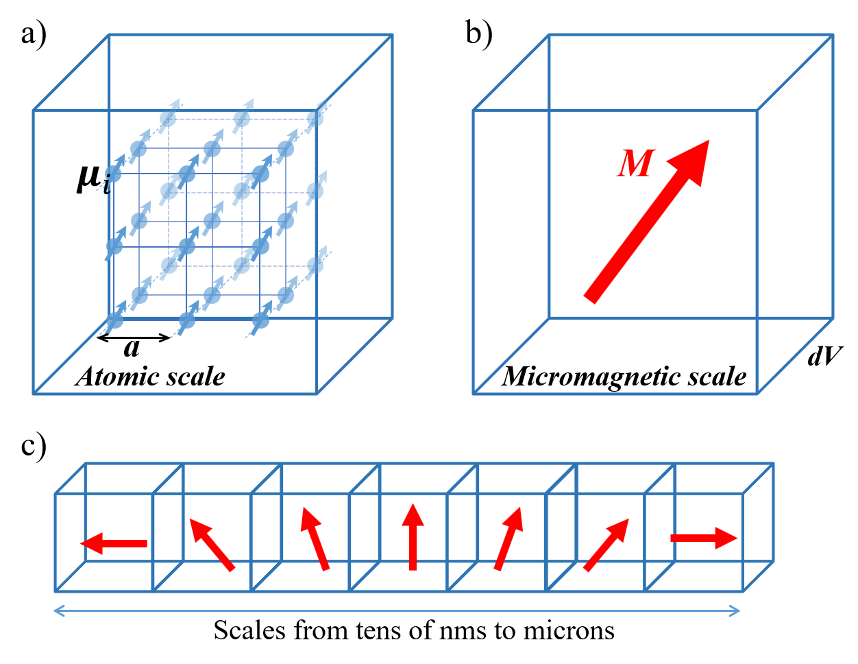Scales in micromagnetism. a) Atomic scale representation of individual magnetic moments \( \boldsymbol{\mu}_i \). b) Micromagnetic scale representation of the magnetization vector \( \boldsymbol{M} \) defining as the sum of all magnetic moments \( \boldsymbol{\mu}_i \) inside the volume \( dV \): \( \boldsymbol{M} = \sum_{i} \boldsymbol{\mu}_i/dV \).

Micromagnetic simulations are based on a set of mathematical equations and models that describe the behavior of magnetic materials. Some of the key concepts and components involved in micromagnetic simulations include Magnetic moments (magnetic materials are divided into small, discretized cells or elements, each having a magnetic moment, which represents the local magnetization of the material. The magnetic moments are usually described as vectors, indicating both the magnitude and direction of the magnetization, see the figure above), Exchange energy (which accounts for the tendency of neighboring magnetic moments to align with each other due to quantum mechanical effects), Anisotropy energy (which describes the directional dependence of a material’s magnetic properties), Zeeman energy (which represents the interaction of the magnetic moments with an externally applied magnetic field), and magnetostatic (dipolar, or demagnetization) interactions. Each magnetic moment is described by the following differential equations:

\[ \frac{d\mathbf{M}}{dt} = -\gamma (\mathbf{M} \times \mathbf{H}_{\text{eff}}) + \frac{\alpha}{M_s} (\mathbf{M} \times \frac{d\mathbf{M}}{dt}) \]

Here, \( \frac{d\mathbf{M}}{dt} \) is the time derivative of the magnetization, \( \gamma \) is the gyromagnetic ratio, \( \mathbf{H}_{\text{eff}}\) is the effective magnetic field (an equaivalent field that includes all the energy terms above), \( \alpha \) is the Gilbert damping parameter, and \( M_s \) is the saturation magnetization of the material.

In micromagnetic simulations, Fast Fourier Transform (FFT) is particularly helpful in calculating magnetostatic interactions.

Magnetostatic interactions are long-range interactions that arise due to the presence of magnetic charges on the surfaces of magnetic domains. These interactions have a significant influence on the overall behavior of magnetic materials, including domain formation, domain wall motion, and magnetization dynamics. Accurate calculation of magnetostatic interactions is crucial for reliable micromagnetic simulations.

Computing magnetostatic interactions directly in the spatial domain can be computationally expensive, especially for large systems or fine discretization grids. However, with FFT, it is possible to perform these calculations more efficiently in the frequency domain. But be careful, even with the use of the FFT, the micromagnetic simulations can still be extremely time-consuming and the calculation of this interaction terms is still the main source of long simulation time: For example for simulation of a spin-torque nano-oscillator with size of ~100 nm, the simulation time could be in the order of minutes to hours without magnetostatic field, and could range from a few hours to a day or more With magnetostatic field (depending on the mesh resolution, simulation settings, and the hardware resources available)

This is also a big problem that I met in my project, and that’s why I started exploring other methods that can help solve this long simulation time problem!

But still, I would like to help you figure out how is demagnetization is calculated with the assistance of the FFT.

Calculation of demagnetization field

The demagnetization field, which can be derived from the Maxwell equation (checkout my thesis for the derivation), can be expressed as (neglecting the coefficient):

\[ \mathbf{H}_\text{demag}(\mathbf{r}) = \int \frac{\rho_m(\mathbf{r’})}{|\mathbf{r} - \mathbf{r’}|^3} (\mathbf{r} - \mathbf{r’}) d\mathbf{r’} \]

where \(\rho_m = -\nabla \cdot \mathbf{M}\) is the charge density. Using the Green’s function (\( G(\mathbf{r}, \mathbf{r’}) = \frac{1}{4\pi|\mathbf{r} - \mathbf{r’}|} \) with its derivative \( \nabla G(\mathbf{r}, \mathbf{r’}) = -\frac{\mathbf{r} - \mathbf{r’}}{4\pi|\mathbf{r} - \mathbf{r’}|^3} \) ), it can be further expressed as:

\[ \mathbf{H}_\text{demag}(\mathbf{r}) = \int{}\nabla G(\mathbf{r}, \mathbf{r’}) \rho_m(\mathbf{r’})dr’ \]

Recalling the formation of Convolution of two functions, we hereby obtain a simplified verion of the expression：

\[ \mathbf{H}_\text{demag}(\mathbf{r}) = \nabla G(\mathbf{r}) * \rho_m(\mathbf{r}) \]

where \(*\) denotes the convolution operation.

The convolution theorem, which establishes a relationship between the convolution operation in the spatial (or time) domain and the multiplication operation in the frequency domain, states that the Fourier Transform of the convolution of two functions is equal to the product of the Fourier Transforms of the individual functions. Therefore, to calculate the demagnetization field, \( \mathbf{H}_\text{demag}(\mathbf{r}) \), we can firstly calculate the convolution of the gradient of the Green’s function, \( \nabla G(\mathbf{r})\), and the magnetic charge density, \( \rho_m(\mathbf{r}) \), which can be expressed as:

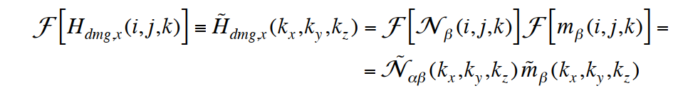
\[ \mathcal{F}{\mathbf{H}_\text{demag}(\mathbf{r})}(\mathbf{k}) = \mathcal{F}{\nabla G(\mathbf{r})}(\mathbf{k}) \cdot \mathcal{F}{\rho_m(\mathbf{r})}(\mathbf{k}) \]

where \( \mathcal{F}{\cdot} \) denotes the Fourier Transform, and \( \mathbf{k} \) represents the frequency domain.

The demagnetization field in the spatial domain can therefore be obtained by applying the inverse Fourier Transform:

\[ \mathbf{H}_\text{demag}(\mathbf{r}) = \mathcal{F}^{-1}{\mathcal{F}{\nabla G(\mathbf{r})}(\mathbf{k}) \cdot \mathcal{F}{\rho_m(\mathbf{r})}(\mathbf{k})} \]

Benefits of transferring to the frequency domain

The benefits of transferring to the frequency doman comes from the advantage of using the FFT algorithm. The naïve approach to compute the convolution of two functions, both having N elements, has a computational complexity of \(O(N^2)\). However, the FFT algorithm computes the discrete Fourier Transform (DFT) of an N-element function in \(O(N \log N)\) time. This computational efficiency also applies to the inverse FFT (IFFT).

Thus, by using the FFT to transform the functions to the frequency domain, perform element-wise multiplication, and then transform the result back to the spatial domain using IFFT, the overall computation is significantly faster compared to the direct computation of the convolution in the spatial domain.

In Micromagnetic simulations, this procedure is done in descretized cells in simulation softwares such as Mumax or OOMMF.

Sorry, I forgot the source of this image, but it shows the descretized version in software

Afterword

Actually, It was when I was writing my PhD thesis I noticed the application of FFT in micormagnetic simulations, I was very surprised about that because FFT is a very old algorithm and I was impressed by the power of this algorithm when I first time learned its working mechanism in the course of Digital Signal Processing in my undergraduate studies. I therefore had the feeling that the past experience can be connected, and we won’t know what impact of the things we are doing will make on the future of us.